Scikit-Learn SpectralEmbedding Model

SpectralEmbedding is a non-linear dimensionality reduction technique that aims to preserve the global structure of the data in a lower-dimensional space. It is particularly useful when the data has a non-linear structure that cannot be effectively captured by linear techniques like PCA.

The key hyperparameters of SpectralEmbedding include n_components (the dimension of the projected subspace), affinity (the kernel used to construct the affinity matrix), and eigen_solver (the eigenvalue decomposition strategy to use).

This algorithm is appropriate for unsupervised learning tasks where the goal is to reduce the dimensionality of the data while preserving its global structure, such as in visualization or as a preprocessing step for other machine learning tasks.

from sklearn.manifold import SpectralEmbedding
from sklearn.datasets import make_swiss_roll
import matplotlib.pyplot as plt

# Generate swiss roll dataset
X, _ = make_swiss_roll(n_samples=1000, noise=0.05, random_state=42)

# Create SpectralEmbedding instance
embedding = SpectralEmbedding(n_components=2)

# Fit the model and transform the data
X_transformed = embedding.fit_transform(X)

# Visualize original and transformed data
fig, (ax1, ax2) = plt.subplots(1, 2, figsize=(10, 5))
ax1.scatter(X[:, 0], X[:, 1], c=X[:, 2], cmap=plt.cm.Spectral)
ax1.set_title("Original Data")
ax2.scatter(X_transformed[:, 0], X_transformed[:, 1], c=X[:, 2], cmap=plt.cm.Spectral)
ax2.set_title("Transformed Data")
plt.tight_layout()
plt.show()

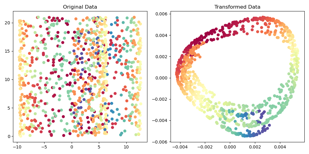
Running the example produces a plot the looks like:

The steps are as follows:

1. First, a synthetic dataset with a non-linear structure (swiss roll) is generated using the make_swiss_roll() function. This creates a 3D dataset with a specified number of samples (n_samples) and a fixed random seed (random_state) for reproducibility.

2. Next, a SpectralEmbedding instance is created with the desired number of output dimensions (n_components) set to 2 for visualization purposes.

3. The fit_transform() method is called on the SpectralEmbedding instance, which fits the model to the data and returns the transformed dataset in the lower-dimensional space.

4. Finally, the original and transformed data are visualized using scatter plots. The color of each point is determined by its position along the third dimension of the original data, which helps to illustrate how the global structure is preserved in the lower-dimensional space.

This example demonstrates how to use SpectralEmbedding to reduce the dimensionality of a dataset with a non-linear structure while preserving its global properties. The transformed data can be used for visualization or as input to other machine learning algorithms that may benefit from working in a lower-dimensional space.