Scikit-Learn LocallyLinearEmbedding Model

Locally Linear Embedding (LLE) is an unsupervised learning algorithm for nonlinear dimensionality reduction. It seeks to preserve the local neighborhood structure of high-dimensional data in a lower-dimensional space.

The key hyperparameters of LLE are the number of neighbors used to define the local structure and the number of components or dimensions in the embedded space. Typical values for neighbors range from 5 to 50, while components are often 2 or 3 for visualization purposes.

LLE is particularly useful for visualizing high-dimensional data in lower dimensions while maintaining the intrinsic structure of the data.

from sklearn.datasets import make_swiss_roll
from sklearn.manifold import LocallyLinearEmbedding
import matplotlib.pyplot as plt

# Generate swiss roll dataset
X, _ = make_swiss_roll(n_samples=1000, noise=0.2, random_state=42)

# Create LLE model
lle = LocallyLinearEmbedding(n_neighbors=12, n_components=2, random_state=42)

# Fit the model to the data
X_lle = lle.fit_transform(X)

# Plot original and transformed data
fig, (ax1, ax2) = plt.subplots(1, 2, figsize=(12, 6))
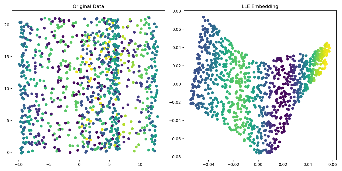
ax1.scatter(X[:, 0], X[:, 1], c=X[:, 2], cmap=plt.cm.viridis)
ax1.set_title('Original Data')
ax2.scatter(X_lle[:, 0], X_lle[:, 1], c=X[:, 2], cmap=plt.cm.viridis)
ax2.set_title('LLE Embedding')
plt.tight_layout()
plt.show()

Running the example produces a plot the looks like:

The steps are as follows:

1. Generate a high-dimensional dataset using make_swiss_roll() from scikit-learn. This creates a 3D swiss roll manifold, which we will aim to unfold into a 2D space.

2. Instantiate an LocallyLinearEmbedding model, specifying the number of neighbors to consider for each point (n_neighbors) and the number of dimensions to embed the data into (n_components).

3. Fit the LLE model to the data using fit_transform(), which learns the manifold structure and returns the transformed dataset X_lle.

4. Visualize the original 3D data and the transformed 2D embedding using matplotlib. The color of each point corresponds to its position along the third dimension in the original data, making it easy to see how the structure is preserved.

This example demonstrates the power of LLE in reducing the dimensionality of complex, nonlinear data while maintaining its local structure. The transformed data can be more easily visualized and interpreted, aiding in understanding the underlying patterns in high-dimensional datasets.