Scikit-Learn learning_curve() to Evaluate Models

learning_curve() is a useful function for understanding the performance of a model relative to the size of the training dataset. It helps in identifying whether the model suffers from high variance or high bias by plotting the training and validation scores.

The learning_curve() function trains the model on different subsets of the training data and evaluates it on the validation set, providing insights into how the training size affects performance. Key hyperparameters include estimator (the model to be trained), train_sizes (the proportion of the dataset to use for generating learning curves), and cv (the cross-validation splitting strategy). This function is suitable for any predictive modeling task such as classification or regression to diagnose model learning behavior.

import numpy as np
import matplotlib.pyplot as plt
from sklearn.datasets import make_classification
from sklearn.model_selection import learning_curve
from sklearn.linear_model import LogisticRegression

# Generate a binary classification dataset
X, y = make_classification(n_samples=1000, n_features=20, n_classes=2, random_state=1)

# Create a Logistic Regression model
model = LogisticRegression()

# Use learning_curve to get train and test scores
train_sizes, train_scores, test_scores = learning_curve(model, X, y, cv=5, train_sizes=np.linspace(0.1, 1.0, 10))

# Calculate mean and standard deviation for plotting
train_scores_mean = np.mean(train_scores, axis=1)
train_scores_std = np.std(train_scores, axis=1)
test_scores_mean = np.mean(test_scores, axis=1)
test_scores_std = np.std(test_scores, axis=1)

# Plot learning curves
plt.figure()
plt.title("Learning Curves (Logistic Regression)")
plt.xlabel("Training Examples")
plt.ylabel("Score")
plt.grid()

# Plot the average training and test scores
plt.fill_between(train_sizes, train_scores_mean - train_scores_std, train_scores_mean + train_scores_std, alpha=0.1, color="r")
plt.fill_between(train_sizes, test_scores_mean - test_scores_std, test_scores_mean + test_scores_std, alpha=0.1, color="g")
plt.plot(train_sizes, train_scores_mean, 'o-', color="r", label="Training score")
plt.plot(train_sizes, test_scores_mean, 'o-', color="g", label="Cross-validation score")

plt.legend(loc="best")
plt.show()

Running the example gives an output like:

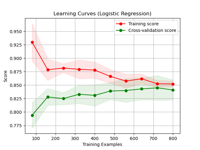
1. First, a synthetic binary classification dataset is generated using the make_classification() function. This creates a dataset with a specified number of samples (n_samples), features (n_features), and a fixed random seed (random_state) for reproducibility.

2. A LogisticRegression model is instantiated.

3. The learning_curve() function is used to compute the training and test scores for different training set sizes with 5-fold cross-validation. This involves training the model on increasingly larger portions of the training data and evaluating the performance on the validation set.

4. The mean and standard deviation of the training and test scores are calculated for plotting.

5. The learning curves are plotted showing the training and cross-validation scores against the number of training examples, providing a visual representation of how the training size impacts model performance.

This example demonstrates how to use learning_curve to visualize the impact of training set size on model performance, helping to diagnose potential issues with bias or variance in the model.