Scikit-Learn GaussianMixture Model

The GaussianMixture model is a probabilistic approach to soft clustering that fits a mixture of multivariate Gaussian distributions to the data. Each Gaussian component represents a cluster, and data points are assigned to clusters based on their probability of belonging to each component.

Key hyperparameters include n_components, which specifies the number of clusters (Gaussian components) to fit, and covariance_type, which determines the type of covariance matrix (e.g., ‘full’, ’tied’, ‘diag’, ‘spherical’).

The algorithm is commonly used for clustering problems and density estimation.

from sklearn.datasets import make_blobs
from sklearn.mixture import GaussianMixture
import matplotlib.pyplot as plt
import numpy as np

# Generate synthetic data
X, y = make_blobs(n_samples=500, centers=3, random_state=42)

# Create GaussianMixture model
model = GaussianMixture(n_components=3, covariance_type='full', random_state=42)

# Fit the model to the data
model.fit(X)

# Plot the decision boundaries
x_min, x_max = X[:, 0].min() - 0.5, X[:, 0].max() + 0.5
y_min, y_max = X[:, 1].min() - 0.5, X[:, 1].max() + 0.5
xx, yy = np.meshgrid(np.arange(x_min, x_max, 0.02),
                     np.arange(y_min, y_max, 0.02))
Z = model.predict(np.c_[xx.ravel(), yy.ravel()]).reshape(xx.shape)

plt.figure()
plt.scatter(X[:, 0], X[:, 1], c=y, cmap='viridis')
plt.contour(xx, yy, Z, colors='black', levels=range(-1, 3))
plt.title("Gaussian Mixture")
plt.show()

# Generate new samples from the model
samples, _ = model.sample(100)
print(samples.shape)

Running the example produces a plot the looks like:

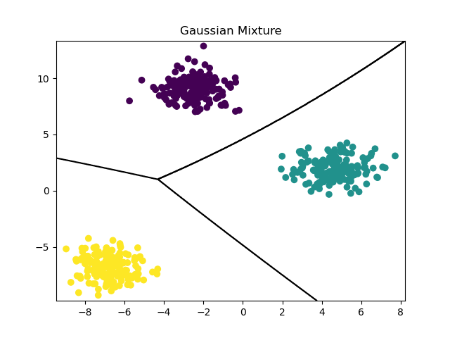
The example follows these key steps:

1. A synthetic dataset suitable for clustering is generated using make_blobs(). This creates a 2D dataset with a specified number of clusters (centers) and samples (n_samples).

2. A GaussianMixture model is instantiated, specifying the desired number of components (n_components) and the covariance matrix type (covariance_type).

3. The model is fit to the data using the fit() method. This learns the parameters of the Gaussian mixture that best models the data distribution.

4. The decision boundaries of the fit model are visualized using plt.contour(). This plots the boundaries where the predicted probabilities of belonging to each cluster are equal.

5. New samples are generated from the learned mixture model using the sample() method. This demonstrates how the model can be used for density estimation and generating new data points that follow the learned distribution.

The GaussianMixture model provides a flexible and probabilistic approach to clustering that can model complex data distributions. The ability to generate new samples from the learned model is a unique feature that distinguishes it from hard clustering algorithms like K-means.