Scikit-Learn fetch_california_housing() Dataset

Datasets

The California Housing dataset consists of housing data collected in 1990 for California. It is commonly used for regression tasks to predict housing prices based on various features like median income and house age.

Key function arguments when loading the dataset include return_X_y to specify if data should be returned as a tuple, and as_frame to get the data as a pandas DataFrame.

This is a regression problem where common algorithms like Linear Regression, Decision Trees, and Random Forests are often applied.

from sklearn.datasets import fetch_california_housing

# Fetch the dataset
dataset = fetch_california_housing(as_frame=True)

# Display dataset shape and types
print(f"Dataset shape: {dataset.data.shape}")
print(f"Feature types:\n{dataset.data.dtypes}")

# Show summary statistics
print(f"Summary statistics:\n{dataset.data.describe()}")

# Display first few rows of the dataset
print(f"First few rows of the dataset:\n{dataset.data.head()}")

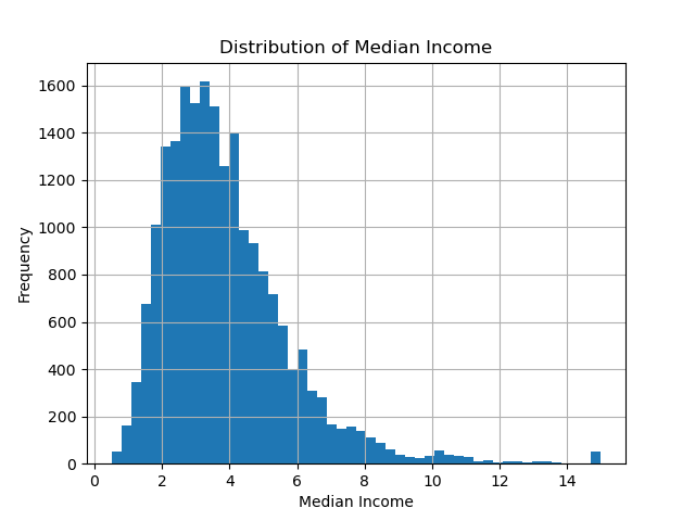
# Example of visualizing the data (e.g., histogram of median income)
import matplotlib.pyplot as plt

dataset.data['MedInc'].hist(bins=50)
plt.xlabel('Median Income')
plt.ylabel('Frequency')
plt.title('Distribution of Median Income')
plt.show()

Running the example gives an output like:

Dataset shape: (20640, 8)
Feature types:
MedInc        float64
HouseAge      float64
AveRooms      float64
AveBedrms     float64
Population    float64
AveOccup      float64
Latitude      float64
Longitude     float64
dtype: object
Summary statistics:
             MedInc      HouseAge  ...      Latitude     Longitude
count  20640.000000  20640.000000  ...  20640.000000  20640.000000
mean       3.870671     28.639486  ...     35.631861   -119.569704
std        1.899822     12.585558  ...      2.135952      2.003532
min        0.499900      1.000000  ...     32.540000   -124.350000
25%        2.563400     18.000000  ...     33.930000   -121.800000
50%        3.534800     29.000000  ...     34.260000   -118.490000
75%        4.743250     37.000000  ...     37.710000   -118.010000
max       15.000100     52.000000  ...     41.950000   -114.310000

[8 rows x 8 columns]
First few rows of the dataset:
   MedInc  HouseAge  AveRooms  ...  AveOccup  Latitude  Longitude
0  8.3252      41.0  6.984127  ...  2.555556     37.88    -122.23
1  8.3014      21.0  6.238137  ...  2.109842     37.86    -122.22
2  7.2574      52.0  8.288136  ...  2.802260     37.85    -122.24
3  5.6431      52.0  5.817352  ...  2.547945     37.85    -122.25
4  3.8462      52.0  6.281853  ...  2.181467     37.85    -122.25

Scikit-Learn fetch_california_housing() Dataset plot

The steps are as follows:

Import the fetch_california_housing function from sklearn.datasets:
- This function allows us to load the California Housing dataset directly from the scikit-learn library.
Fetch the dataset using fetch_california_housing():
- Use as_frame=True to return the dataset as a pandas DataFrame for easier data manipulation and analysis.
Print the dataset shape and feature types:
- Access the shape using dataset.data.shape.
- Show the data types of the features using dataset.data.dtypes.
Display summary statistics:
- Use dataset.data.describe() to get a statistical summary of the dataset.
Display the first few rows of the dataset:
- Print the initial rows using dataset.data.head() to get a sense of the dataset structure and content.
Visualize the distribution of median income:
- Plot a histogram of the MedInc (Median Income) feature using matplotlib to understand its distribution.

This example demonstrates how to quickly load and explore the California Housing dataset using scikit-learn’s fetch_california_housing() function, allowing you to inspect the data’s shape, types, summary statistics, and visualize a key feature. This sets the stage for further preprocessing and application of regression algorithms.

See Also